At TechEd 2013, I attended a few sessions on the topics of Data Mining and Predictive Analytics.  I thought I’d try out the data mining functionality in SSAS using warranty data from a data mart to predict the quantities of failed parts over the next few months.   To accomplish this, I created a Data Mining structure in SSAS using the Microsoft Time Series Algorithm.  This is my first attempt at data mining, so I thought I’d write a blog post to document what I’ve learned so far.

As a first step, I needed to structure my data in a format that is compatible with the Time Series Algorithm.  The following are requirements of the time series model:

• Key time / date column: The model must contain one numeric or date column that specifies the time slices.  The column must contain continuous values and the values must be unique for each series.
• Predictable column: The model must contain at least one predicable column, the data type of this column must store continuous values.
• Series key column: The model can also include an optional additional key column.  This column must contain unique values that identify a series.

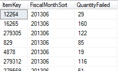
I created a table (named DataMining_Test) that consists of three columns:

• FiscalMonthSort: Key time/date column.  The data is in the format YYYYMM.
• ItemKey: Series key column, stores a numeric value that specifies a unique part/item.
• QuantityFailed: Predictable column.

The following is a sample of the data:

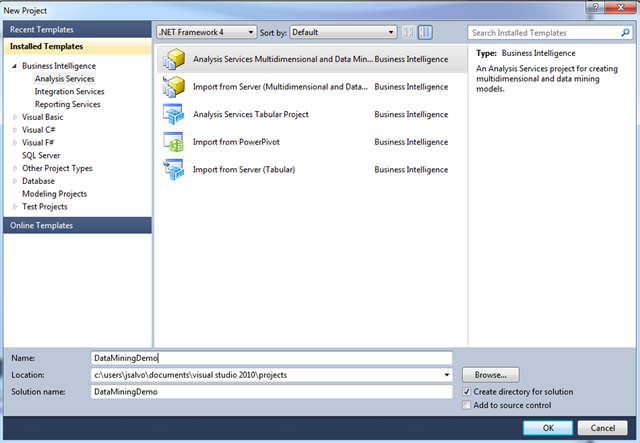
Next, I created a new SSAS Data Mining project in SSDT (formerly BIDS).  To create a SSAS project, click File > New > Project and select the option labeled ‘Analysis Services Multidimensional and Data Mining’.  Click ‘OK’.

As a first step, you’ll need to create a new Data Source that stores the data you need for data mining.  Right click on ‘Data Sources’ and fill in the necessary details to create your data source.

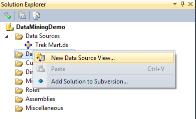
Next, create a new ‘Data Source View’.  Right click on Data Source Views and then click ‘New Data Source View’.

Complete the steps of the wizard, be sure to add the table that stores the data needed for data mining to the Data Source View.

Once you’ve created your Data Source and Data Source View, you can now create a Mining Structure.

To create a Mining Structure, right click on ‘Mining Structures’ and select ‘New Mining Structure’.  You’ll then see the wizard below.

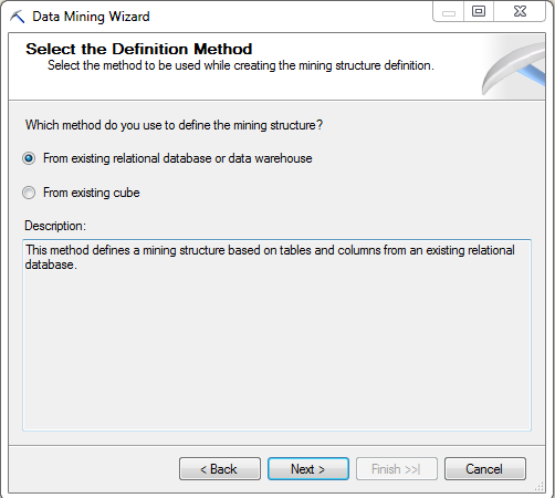
Now you must select a method to define the mining structure.  You have two options: ‘Existing relational database/data warehouse’ or ‘Existing cube’.  In this example, the data is stored in a relational table so I selected ‘From existing relational database or data warehouse’. 

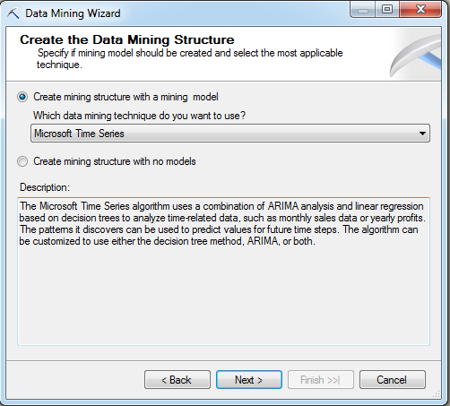
Now you must select the type of mining technique you wish to use.  In this example, I will choose the option labeled ‘Microsoft Time Series’.

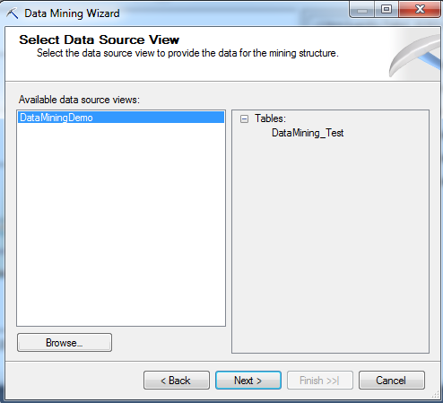
Now select your data source view.  In this example, my data source view is called DataMiningDemo and it consists of one table named DataMining_Test.

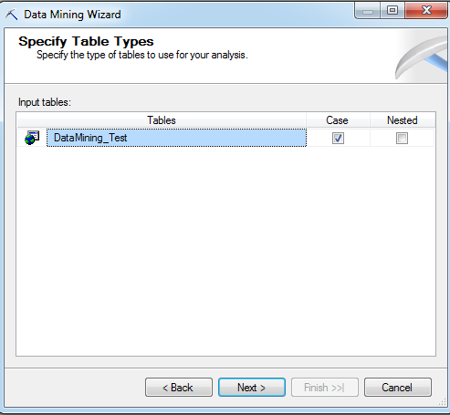
You must also specify the table(s) that store the data for the data mining analysis.

Now you must indicate if a column is a key, an input or predictable. 

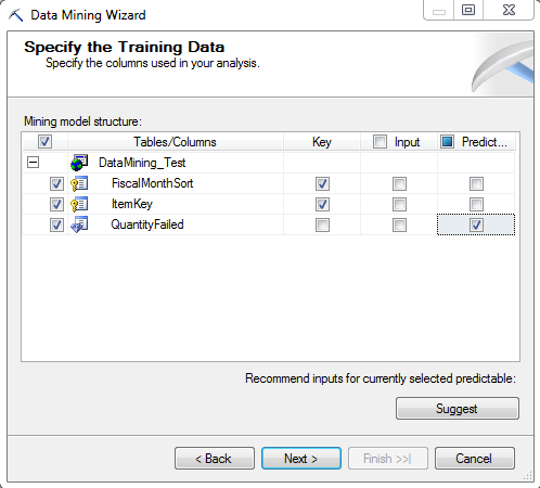
The columns named FiscalMonthSort and ItemKey are marked as Key columns, while QuantityFailed is marked as Predictable.

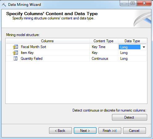
You have the option to change the data type of each column, if needed.

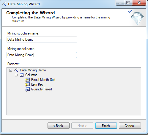
Finally, give your Mining Model a name and click ‘Finish’.

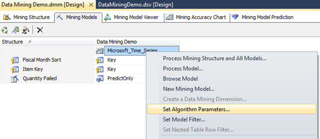
Now that we’ve created the Mining Model, we must set the Mining Model parameters.  To set parameters, click on the ‘Mining Models’ tab and right click on the name of your Mining Model.  Select the option ‘Set Algorithm Parameters’.

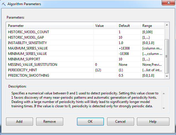
In this example, the PERIODICITY_HINT should be set to {12} since the data is broken down into months.  MISSING_VALUE_SUBSTITUTION is set to 0, this value is used to fill in any gaps/missing data in the historical data set.  We will leave all other parameters set to the default value.

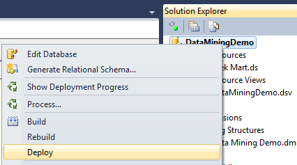
Now, you need to deploy and process your Mining Model.  In this example, I have configured my project to fully process the mining model when the project is deployed to an instance of Analysis Services.  To deploy the project, right click on the project name and select ‘Deploy’.

Once you’ve deployed and processed the model, you can view charts that display the past and predicted trends for each series by clicking on the ‘Mining Model Viewer’ tab in SSDTs.  In this example, each series represents an item/part and the prediction is failed quantity.  Below is an example of the chart with a single item selected.

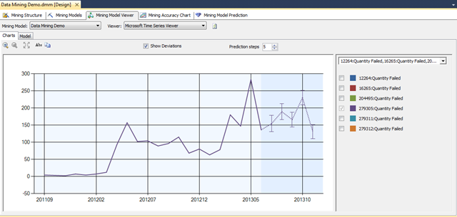
I checked ‘Show Deviations’ to see the confidence interval for each prediction (displayed as bars on the graph).  The smaller the bar, the more confident the prediction.  You can adjust the number of predictions shown in the chart by modifying the ‘Prediction steps’ value.

Now, we can connect to our Mining Model in SSMS to run a prediction query.  Launch SSMS and connect to the instance of Analysis Services with the Mining Model.

Create a new ‘Analysis Services DMX Query’.  In this example, we will predict the failed quantity over the next 6 months by Item Number.  The DMX query is shown below:

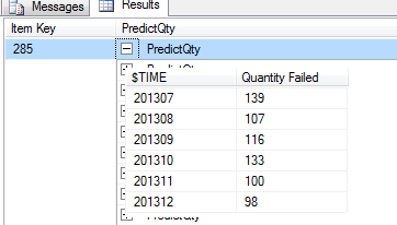
The query produced the following output:

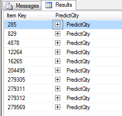
You can expand the PredictQty for any item to see the predicted failed quantity over the next 6 months.

comments powered by Disqus